Overview
In this tutorial we will walk you through all the steps of generating and analyzing OAR scores from your single cell dataset. We will begin with a Seurat object with plasmacytoid dendritic cells that you can download from our github repository.
The process starting from a gene expression matrix is very similar and you should be able to adapt this workflow to that input. Skip a few lines down to the data pre-processing step to run the tutorial that way.
At the end, we provide an alternative single line wrapper function
that runs the whole process, and adds the results to the
meta.data slot of a Seurat object. If starting from a
dataset with multiple cell types or where a biological perturbation
greatly alters gene expression, we recommend running this process
splitting the data by that factor, and similarly provide a wrapper
function that accomplishes that.
1. Loading and pre-processing your data
First, we load a Seurat object that we wish examine and store the cell barcodes so we can later assign them to our output.
sc.data <- readRDS(file = "pdcs.rds")
cells = colnames(sc.data)
sc.data
#> An object of class Seurat
#> 14362 features across 1243 samples within 1 assay
#> Active assay: RNA (14362 features, 2000 variable features)
#>  1 layer present: counts
#>  2 dimensional reductions calculated: pca, umap
Now lets set a count threshold where we only analyze genes expressed in at least 1% of cells1. We do not recommend using thresholds higher than 4%, as information will be lost.
tr = 1Next, we retrieve the un-normalized count data from the Seurat
object, filter low abundance genes and remove genes that are
uninformative2. The output of this function is a list with
the first element being the processed matrix and the second the list of
genes in that matrix after filtering. We will skip the later for this
tutorial. Zero-counts in the processed matrix are denoted as
NA.
oar_data <- oar_preprocess_data(
  data = sc.data, tr = tr,
  seurat_v5 = T, blacklisted.genes = NULL)
#> [1] "Extracting count tables"
oar_data[[1]][1:5,1:5]
#>      [,1] [,2] [,3] [,4] [,5]
#> [1,]   NA    1   NA    1   NA
#> [2,]   NA   NA   NA   NA   NA
#> [3,]   NA   NA    1   NA   NA
#> [4,]   NA   NA   NA   NA   NA
...
For a full description of each parameter consult the documentation. Briefly:
-
seurat_v5confirms the type of data being used. Defaults toTRUE. If starting from a data matrix, set this toFALSEand continue with the rest of the tutorial. -
trcontrols the minimum percentage of cells expressing any given gene for that gene to be retained in the analysis. Defaults to 1. -
blacklisted.genesallows you to provide a vector of uninformative gene names (i.e. non-coding genes) to exclude from the analysis. Defaults toNULL.
2. Identifying gene co-expression patterns
Our scoring relies on defining gene co-expression patterns based on a
binarized count matrix. To do this, we can identify genes with minimal
mismatch between them, but we need to first enable R to run in parallel.
To determine how many thread are available in your computer, you can run
parallelly::availableCores(). Leave at least 1-2 cores
available for other processes running in your computer to prevent
crashing. Using multiple cores is recommended as pattern identification
will go much faster.
parallelly::availableCores()
#> system
#>      4
Now we can select an appropriate number to set up parallel processing for this R session. To identify patterns allowing for mismatch, we calculate the hamming distance between all pairs of gene expression vectors. Internally, the gene vectors are converted to 0 (absent) and 1 (expressed) values. This function needs to have the number of cores specified explicitly.
dm <- oar_hamming_distance(
  oar_data[[1]], cores = 1)
#> [1] "Calculating Hamming distances between gene vectors using specified cores."
#> [1] "This operation may take several minutes"
#> OpenMP reports: max_threads = 1, num_procs = 4, actual used = 1
#> OpenMP reports: max_threads = 1, num_procs = 4, actual used = 1
#> OpenMP reports: max_threads = 1, num_procs = 4, actual used = 1
...
dm[[1]][1:5,1:5]
#>            1          2          3          4          5
#> 1 0.00000000 0.02976669 0.02976669 0.02815768 0.02976669
#> 2 0.02976669 0.00000000 0.03218021 0.02896219 0.03378922
#> 3 0.02976669 0.03218021 0.00000000 0.02735318 0.03218021
#> 4 0.02815768 0.02896219 0.02735318 0.00000000 0.02896219
...
The output is a list of matrices, with each matrix containing a set
of genes grouped based on overall sparsity, and where the hamming
distance between pairs of gene expression vectors within each matrix is
calculated. Expression binning is introduced to increase computational
performance and introduce a dynamic threshold to identify patterns. In
the wrapper function oar you have the possibility of
storing this result in your Seurat object, so that future score
calculations are completed faster. The wrapper function automatically
detects a previously calculated hamming distance matrix and uses that
for further analysis. WARNING: If you use a different count
filter value, or a different set of cells, these distances will no
longer be appropriate. In that case, remove previously calculated
distance matrix using
oar_obj[["RNA"]]@misc <- list().
Next, we want to group genes into co-expression patterns based on a minimal hamming distance threshold.
gcp <- oar_patterns(oar_data[[1]], dm)
#> [1] "Identified 24 gene co-expression patterns"
#> [1] "A total of 331 genes captured in co-expression patterns"
table(gcp)
#> gcp
#>  ptn.1 ptn.10 ptn.11 ptn.12 ptn.13 ptn.14 ptn.15 ptn.16 ptn.17 ptn.18 ptn.19
#>    108      2     30      2      3      4      2      3      4      3      5
#>  ptn.2 ptn.20 ptn.21 ptn.22 ptn.23 ptn.24  ptn.3  ptn.4  ptn.5  ptn.6  ptn.7
#>     12      2      2      5      2      2     39     21     31      2      2
...
A few considerations on pattern matching: Allowing
only for exact matches results in very few, and often no, co-expressed
gene patterns, which is why our method makes this process more flexible.
Internally, each gene expression bin is assigned a separate minimal
hamming distance threshold (minimum of 0.01), which is used to generate
an adjacency matrix for all genes. Then a graph is built based on this
matrix and the eccentricities of all nodes calculated. Then the minimal
hamming distance threshold is adjusted to cap the eccentricity of all
nodes to maintain pattern integrity. We recommended you plot
KW.BH.pvalue vs. sparsity to examine the
results. You should observe no relationship between these variables,
other than higher p values in some - but not all -
cells with a high sparsity (defined here as a percentage of genes with 0
counts within each cell).
We can visualize these results of the pattern search by using:
p3 <- oar_gcp_plot(data = oar_data[[1]], gcp = gcp, seurat_v5 = FALSE)
#> [1] "Generating plots..."
p3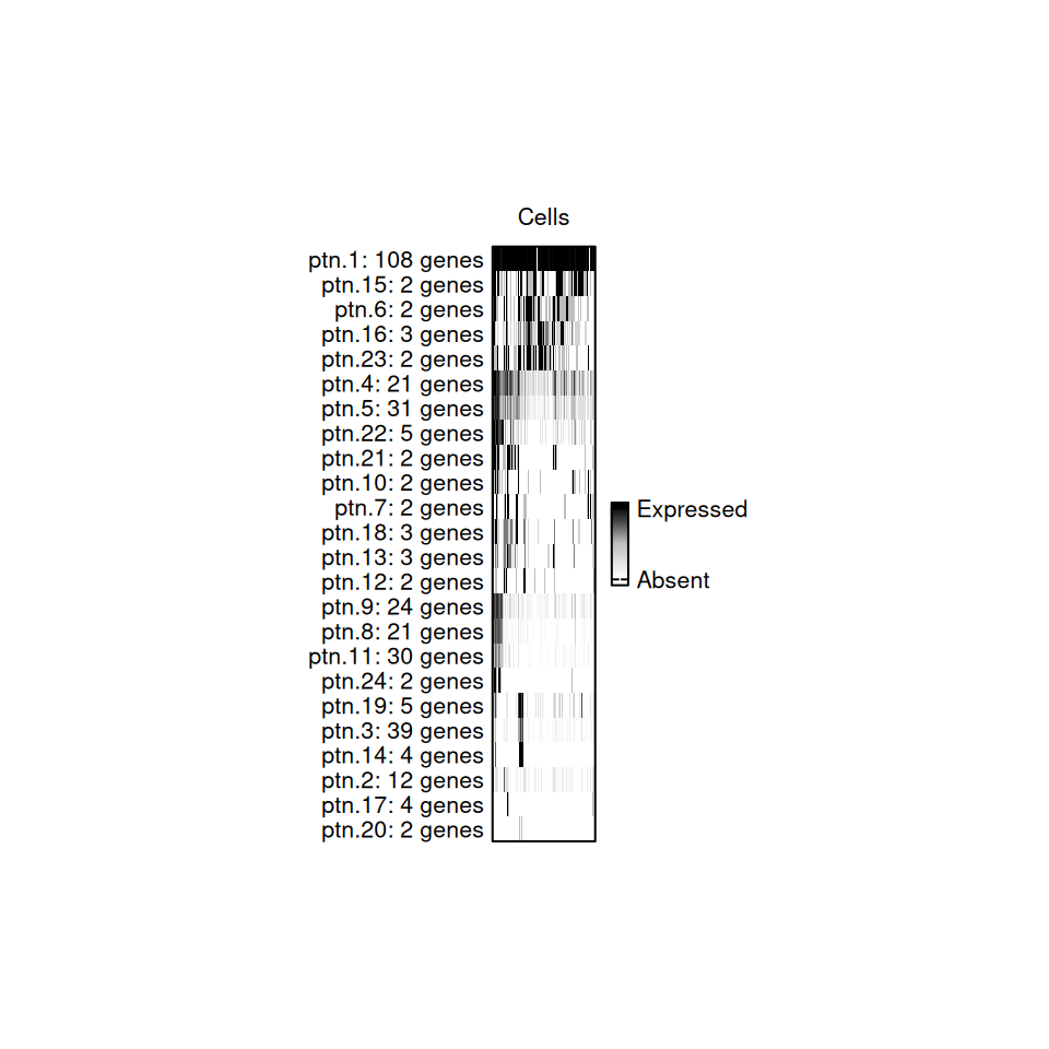
Gene co-expression patterns Plot
Each slice of the bar represents a cell, and it is colored based on what percentage of genes from that pattern are expressed in each cell.
3. Calculate OAR scores
Now we are ready to do a cell-wise estimation of the overlap between the gene expression distributions in each detected pattern. When these distributions are distinct we obtain a highly significant p value and an OAR score of less than 2. Alternatively, when these distributions overlap cells have a larger p value and an OAR score greater than 2. Thus, a cell where the patterns defined in the whole dataset do not explain gene expression, will have a with a high OAR score and is potentially distinct from all others. Critically, our test incorporates both the gene expression values and the gene co-expression patterns.
output <- oar_base(data = oar_data[[1]], gcp = gcp)
output$barcodes = cells #add back our barcodes
output
#>           OARscore    KW.pvalue KW.BH.pvalue sparsity             barcodes
#> 1     0.4991194964 1.310249e-74 1.672114e-74 79.46352 AAACCTGAGAACAATC-1_1
#> 2    -0.5335102274 9.891672e-83 3.595131e-82 87.92927 AAACCTGAGGTGCTAG-1_1
#> 3    -1.0294046721 7.161214e-87 7.474225e-86 85.27251 AAACCTGGTAGCAAAT-1_1
#> 4    -1.3317223078 2.258655e-89 4.253800e-88 78.79720 AAACGGGGTACCCAAT-1_1
...
The result is a matrix with these columns:
-
OARscoreis a metric of transcriptional shifts in the data, with a higher OAR score highlighting cells with gene expression patterns dissimilar from all others tested. -
KW.pvalueis the p-value generated by Kruskal-Wallis test. -
KW.BH.pvalueis the Benjamini-Hochberg corrected p-value. -
sparsityis the percent of genes in each cell with a count of 0.
We can now proceed to visualize these results to identify which cells display transcriptional shifts.
4. Visualize results
A higher OAR score is a way to prioritize cells for further analysis. Greater scores indicate distinct cell expression signatures, where high scoring cells have different gene co-expression patterns compared to all other cells in the test. In this example, we observe that cells with a high degree of sparsity, also have a high OAR score
library(ggplot2)
p1 <-ggplot(
  data = output,
  aes(x = sparsity,
      y = OARscore,
      color = -log10(KW.BH.pvalue))) +
  geom_point(size = 0.5) +
  labs(
    x = "Sparsity (%)",
    y = "OAR score") +
  geom_hline(
    yintercept = 2, linetype = "dashed",
    color = "black", linewidth = 0.25) +
  scale_colour_gradientn(
    colours = (c("#000004FF","#3B0F70FF","#8C2981FF",
                    "#DE4968FF", "#FE9F6DFF","#FCFDBFFF")),
    na.value = "transparent",
    name = expression(-Log[10]~BH.pval),
    guide = guide_colorbar(
      frame.colour = "black",
      frame.linewidth = 0.2,
      ticks.linewidth = 0.2,
      ticks.colour = "black")) +
  theme(
    aspect.ratio = 1,
    panel.grid = element_blank(),
    panel.background = element_blank(),
    axis.line = element_line(linewidth = 0.5),
    legend.text = element_text(size = 6),
    legend.title = element_text(size = 8),
    legend.key.size = unit(3, "mm"),
    axis.text = element_text(size = 6),
    axis.title = element_text(size = 8),
    plot.title = element_blank())
p1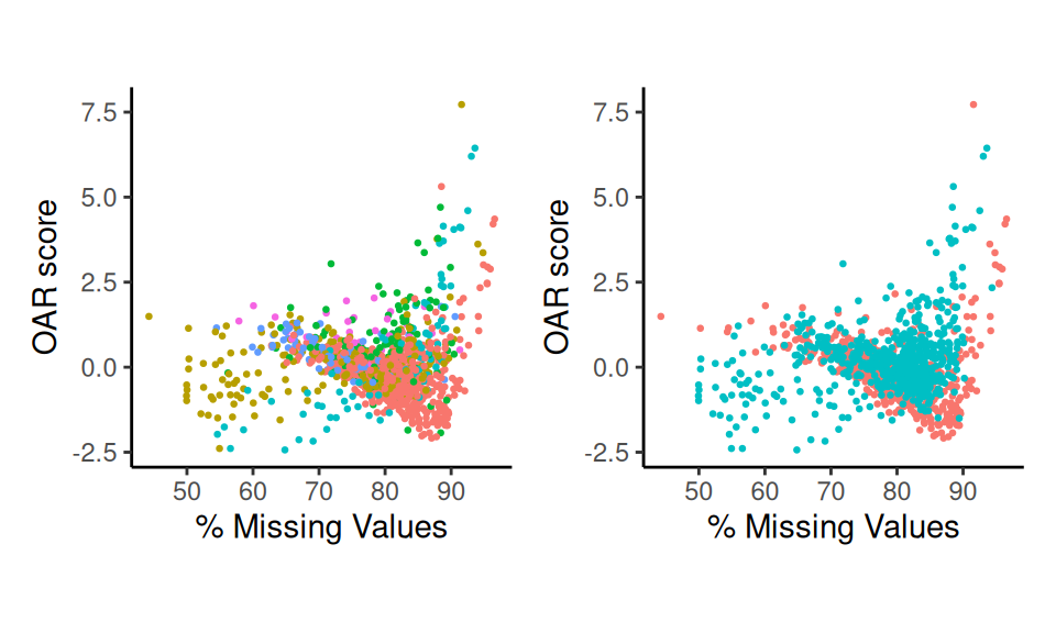
Scatter Plots
You may recreate this plot using scatter_score().
In order to fully understand the features in the dataset driving the high OAR score in some cells, it will be necessary to annotate these with their biological context. This is more easily achieved within a Seurat object with the additional experimental details.
5. Wrapper functions and result interpretation
We can run this entire process with a single line. The result is the
Seurat object with the OARscore, KW.pvalue,
KW.BH.pvalue and sparsity values in the
meta.data slot. Additionally, genes are annotated by which
gene co-expression patterns they have been included in
sc.data@assays$RNA@meta.data.
sc.data <- oar(data = sc.data,
               seurat_v5 = T, count.filter = 1,
               blacklisted.genes = NULL, suffix = "",
               store.hamming = T,
               cores = 1)
#> Warning in oar(data = sc.data, seurat_v5 = T, count.filter = 1, blacklisted.genes = NULL, : Running process in fewer than 2 cores will considerably slow down progress
#> [1] "Extracting data..."
#> [1] "Extracting count tables"
#> [1] "Analysis started on:"
#> [1] "2026-03-26 16:28:45 UTC"
#> [1] "Identifying gene co-expression patterns..."
...
We set these parameters based on our earlier discussion:
-
seurat_v5confirms the type of data being used. Defaults toTRUE. -
count.filtercontrols the minimum percentage of cells expressing any given gene for that gene to be retained in the analysis. Defaults to 1. -
blacklisted.genesAllows you to provide a vector of uninformative gene names (i.e. non-conding genes) to exclude from the analysis. Defaults toNULL. -
suffixAllows you to provide a character string to avoid overwriting previous OAR calculations. Defaults toNULL. -
store.hammingallows you to store the calculated hamming distances for pattern matching in your Seurat object for faster re-calculation of the scores if you need to alter other parameters later (found inoar_obj[["RNA"]]@misc). Defaults toTRUE.
You can use a similar approach to analyse the data cluster by cluster
- recommended when you have multiple cell types - or separated by
another variable in your data. In that case, use
oar_by_factor() and see vignette("OAR_Factor")
for more details.
Interpreting high OAR scores
To explore which cells/clusters display transcriptional shifts, we
can project the scores to our UMAP using
Seurat::FeaturePlot(). Notice that cells with a high OAR
score in this dataset cluster together. In fact, in this case, high OAR
scoring cells represent the most activated cells in the experiment, as
can be seen when we examine IFNA1, which is expressed in
activated plasmacytoid dendritic cells.
library(Seurat)
#> Loading required package: SeuratObject
#> Loading required package: sp
#> 'SeuratObject' was built under R 4.5.0 but the current version is
#> 4.5.3; it is recomended that you reinstall 'SeuratObject' as the ABI
#> for R may have changed
#>
#> Attaching package: 'SeuratObject'
#> The following objects are masked from 'package:base':
#>
#>     intersect, t
p1 <- FeaturePlot(
  sc.data, features = c("OARscore","IFNA1"), order = T, pt.size = 0.5,
  min.cutoff = "q40", max.cutoff = "q90", slot = "counts")
p1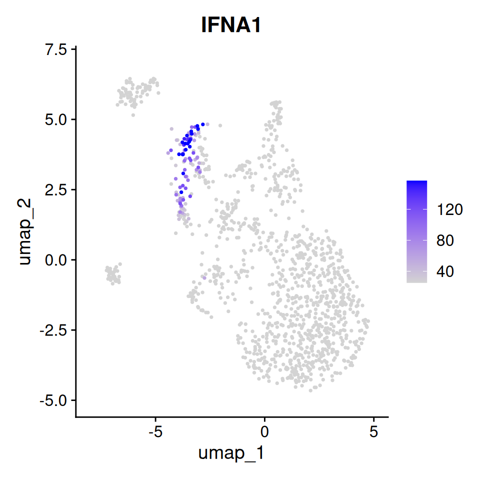
Feature plot of OAR score
Thus, in this dataset we are able to identify highly activated cells
with a cluster agnostic approach. We provide additional tutorials to
identify genes associated with a high OAR score (see:
vignette("Gene_expression")). We have also seen datasets
where high scores are associated with biological variation that may be
removed from the analysis to glean additional insights into the
populations of cells studied. These can be achieved by passing
OARscore to vars.to.regress in
Seurat::SCTransform().