Overview
In this tutorial we will walk you through generating OAR scores from your single cell dataset separated by a factor in your data. We will begin with a Seurat object with Dictyostelium discoideum cells (dicty) that you can download from our github repository.
This approach is usually recommended when you have multiple cell types in your dataset or your experimental conditions introduce dramatic shifts in gene expression patterns. Our approach works best to detect trasncriptional shifts within a set of cells that you expect to be somewhat similar. Consequently, in situations like the ones outlined above, it makes more sense to split the data by a factor before running the analysis.
First, we will take a look at how the test performs when the data is not split. Later we will run the analysis split by factors. As always, we begin by loading the seurat object with the dataset we are interested in.
library(Seurat)
#> Loading required package: SeuratObject
#> Loading required package: sp
#> 'SeuratObject' was built under R 4.5.0 but the current version is
#> 4.5.3; it is recomended that you reinstall 'SeuratObject' as the ABI
#> for R may have changed
#>
#> Attaching package: 'SeuratObject'
#> The following objects are masked from 'package:base':
#>
#>     intersect, t
sc.data <- readRDS(file = "dicty.rds")
sc.data
#> An object of class Seurat
#> 13206 features across 5000 samples within 1 assay
#> Active assay: RNA (13206 features, 2000 variable features)
#>  1 layer present: counts
#>  1 dimensional reduction calculated: umap
1. Running the full test
We can run the full test entire process with a single line. For a
description of all these parameters see our other vignettes. The result
is the Seurat object with the OARscore,
KW.pvalue, KW.BH.pvalue and
sparsity values in the meta.data slot.
sc.data <- oar(data = sc.data,
               seurat_v5 = T, count.filter = 1,
               blacklisted.genes = NULL, suffix = "",
               store.hamming = F,
               cores = 1)
#> Warning in oar(data = sc.data, seurat_v5 = T, count.filter = 1, blacklisted.genes = NULL, : Running process in fewer than 2 cores will considerably slow down progress
#> [1] "Extracting data..."
#> [1] "Extracting count tables"
#> [1] "Analysis started on:"
#> [1] "2026-03-26 16:30:48 UTC"
#> [1] "Identifying gene co-expression patterns..."
...
To explore the results we can visualize OARscore vs
sparsity values, coloring the cells based on some of the
attributes in our Seurat object meta.data.
library(patchwork)
library(ggplot2)
p1 <- scatter_score(sc.data, pt.size = 0.5)+NoLegend()
p2 <- scatter_score(sc.data, pt.size = 0.5, group.by = "group")
p1+p2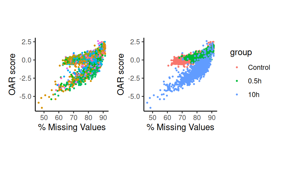
Scatter Plots by Factors
Here we can see that the underlying biological conditions are resulting in very different sets of OARscores. In particular, 10h of starvation, induces a completely separate profile of values. For that reason, running the test separating the data by this biological variable will allow us to prioritize cells within each condition for further analysis.
2. Analysis by Factor
OAR scores are typically more informative when distinguishing among cells of the same type. When working with a dataset with diverse cell types or dramatically affected by a biological variable, it can be helpful to split the data by that factor and run the test independently. This can be easily accomplished with our wrapper function, which takes the same parameters as we have discussed before and returns a Seurat object containing the results of the analysis.
sc.data <- oar_by_factor(sc.data, cores = 1, factor = "group", suffix = ".factor")
#> [1] "Splitting data by specified factor..."
#> Warning in FUN(X[[i]], ...): Running process in fewer than 2 cores will considerably slow down progress
#> [1] "Extracting data..."
#> [1] "Extracting count tables"
#> [1] "Analysis started on:"
#> [1] "2026-03-26 16:31:05 UTC"
#> [1] "Identifying gene co-expression patterns..."
...
#> Warning in FUN(X[[i]], ...): Running process in fewer than 2 cores will considerably slow down progress
#> [1] "Extracting data..."
#> [1] "Extracting count tables"
#> [1] "Analysis started on:"
#> [1] "2026-03-26 16:31:14 UTC"
#> [1] "Identifying gene co-expression patterns..."
...
#> Warning in FUN(X[[i]], ...): Running process in fewer than 2 cores will considerably slow down progress
#> [1] "Extracting data..."
#> [1] "Extracting count tables"
#> [1] "Analysis started on:"
#> [1] "2026-03-26 16:31:18 UTC"
#> [1] "Identifying gene co-expression patterns..."
...
Now let us examine the outcome of this analysis:
p3 <- scatter_score(sc.data, pt.size = 0.5, suffix = ".factor")+NoLegend()
p4 <- scatter_score(sc.data, pt.size = 0.5, group.by = "group", suffix = ".factor")
p3+p4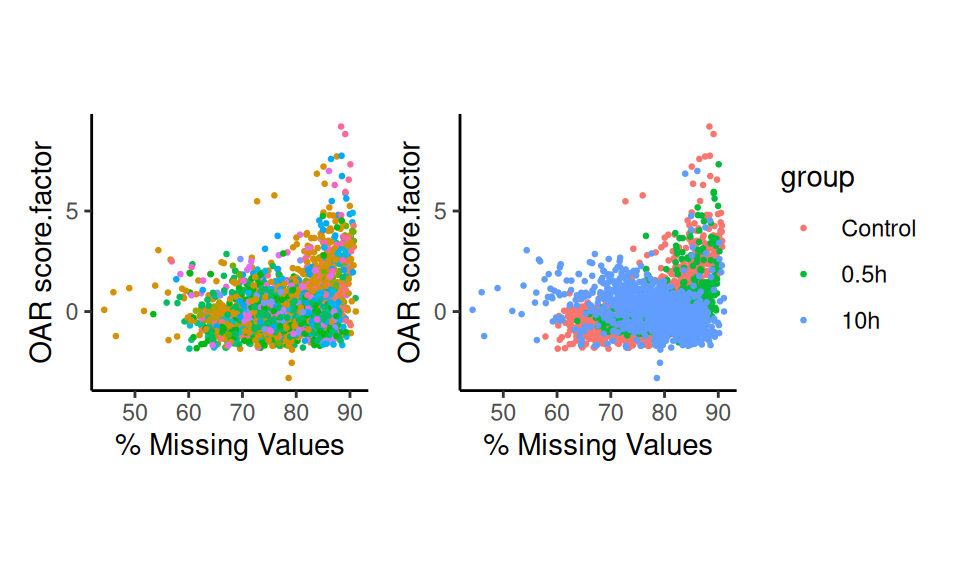
Scatter Plots by Factors
As you can see, we are able to identify trasncriptional shifts within
each biological condition. Moreover, we can visualize these results in a
UMAP projection of the using Seurat::FeaturePlot().
p5 <- FeaturePlot(
  sc.data, features = "OARscore.factor", order = T, pt.size = 0.5,
  min.cutoff = "q40", max.cutoff = "q90")
p5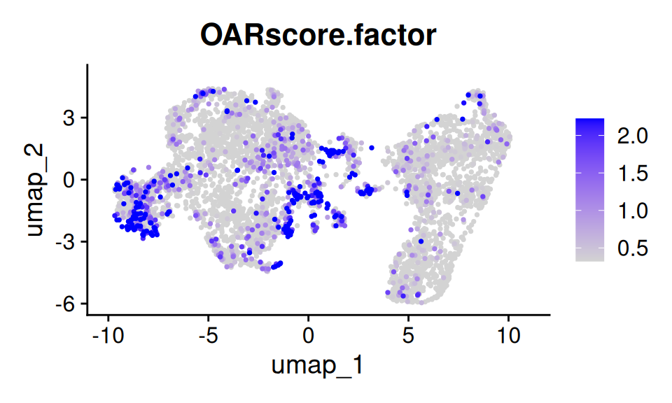
Results by factor