Introductory Vignette for OARscRNA
Source:vignettes/introductory_vignette.Rmd
introductory_vignette.RmdOverview
In this vignette we will walk you through the very basic steps of generating and analyzing OAR scores from your single cell dataset.
There are two possible starting points:
- Seurat v5 Object
- Gene Expression Matrix
Here we will walk you through steps of the analysis, beginning with a gene expression matrix from plasmacytoid dendritic cell dataset that you can download from our github repository.
Starting from v5 Seurat Object
Analysis
We can directly input a Seurat object to examine transcriptional shifts.
data_obj <- readRDS(file = "pdcs.rds")
data_obj
#> An object of class Seurat
#> 14362 features across 1243 samples within 1 assay
#> Active assay: RNA (14362 features, 2000 variable features)
#>  1 layer present: counts
#>  2 dimensional reductions calculated: pca, umap
Once you have the seurat version 5 object loaded, you can run the oar function. This function requires the input data, as well as some information on the number of cores (which is set to 1 by DEFAULT).
To determine how many threads are available for the analysis, you can
run parallelly::availableCores(). Leave at least 1-2 cores
available for other processes running in your computer to prevent
crashing. Using multiple cores is recommended as pattern identification
will go much faster.
oar_obj <- oar(data_obj, cores = 1)
#> Warning in oar(data_obj, cores = 1): Running process in fewer than 2 cores will considerably slow down progress
#> [1] "Extracting data..."
#> [1] "Extracting count tables"
#> [1] "Analysis started on:"
#> [1] "2026-03-26 16:30:20 UTC"
#> [1] "Identifying gene co-expression patterns..."
...
We deliberately left most parameters to their default values, however we recommend you explore each to familiarize yourself with their impact on the result. Some critical parameters to consider include:
-
seurat_v5confirms the type of data being used. Defaults toTRUE. -
count.filtercontrols the minimum percentage of cells expressing any given gene for that gene to be retained in the analysis. Defaults to 1. -
blacklisted.genesallows you to provide a vector of uninformative gene names (i.e. non-coding genes) to exclude from the analysis. Defaults toNULL. -
store.hammingallows you to store the calculated hamming distances for pattern matching in your Seurat object for faster re-calculation of the scores if you need to alter other parameters later (found inoar_obj[["RNA"]]@misc). Defaults toTRUE.
The result is a Seurat object with these additional metadata columns:
-
OARscoreis a metric of transcriptional shifts in the data, with a higher OAR score highlighting cells with gene expression patterns dissimilar from all others tested. -
KW.pvalueis the p-value generated by Kruskal-Wallis test. -
KW.BH.pvalueis the Benjamini-Hochberg corrected p-value. -
sparsityis the percent of genes in each cell with a count of 0.
Additionally, genes are annotated by which gene co-expression pattern they have been included in. This matrix is added to the assay metadata (found in oar_obj@assays$RNA@meta.data).
Analysis by Factor
OAR scores are typically more informative when distinguishing among
cells of the same type. When working with a dataset with diverse cell
types or dramatically affected by a biological variable, it can be
helpful to split the data by that factor and run the test independently.
See vignette("OAR_Factors") for more details.
oar_obj_byfactor <- oar_by_factor(data_obj, cores = 1, factor = "ident")This functions takes the same parameters as oar, but it
will not store the calculated hamming distances in the resulting Seurat
object.
Visualize Results
Below are a few examples of how you might explore the results of this analysis.
OARscore v Sparsity Scatter Plot
library(patchwork)
library(ggplot2)
p1 <- scatter_score(oar_obj, pt.size = 0.5)+theme(legend.position = "none")
p2 <- scatter_score(oar_obj, pt.size = 0.5, group.by = "condition")+theme(legend.position = "none")
p1+p2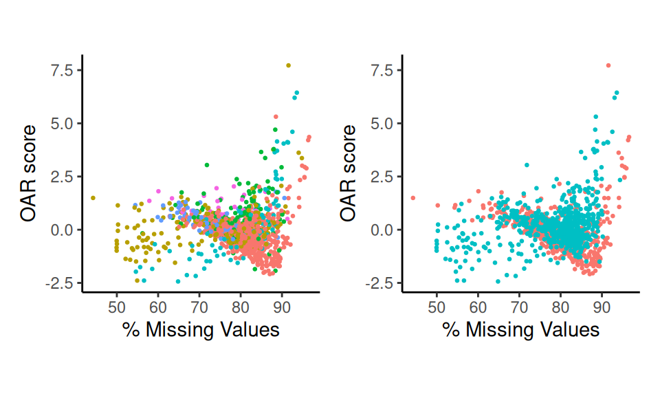
Scatter Plots
These plot reveals which clusters have the highest OAR scores, as
well as how the score relates to sparsity. Adjust the
group.by metric to examine other variables.
Gene co-expression Patterns
In some cases, you might want to explore the patterns that were identified during the analysis to understand what the co-expression gene modules are telling you. First, you can visualize these patterns like this:
p3 <- oar_gcp_plot(oar_obj)
#> [1] "Extracting count tables"
#> [1] "Generating plots..."
p3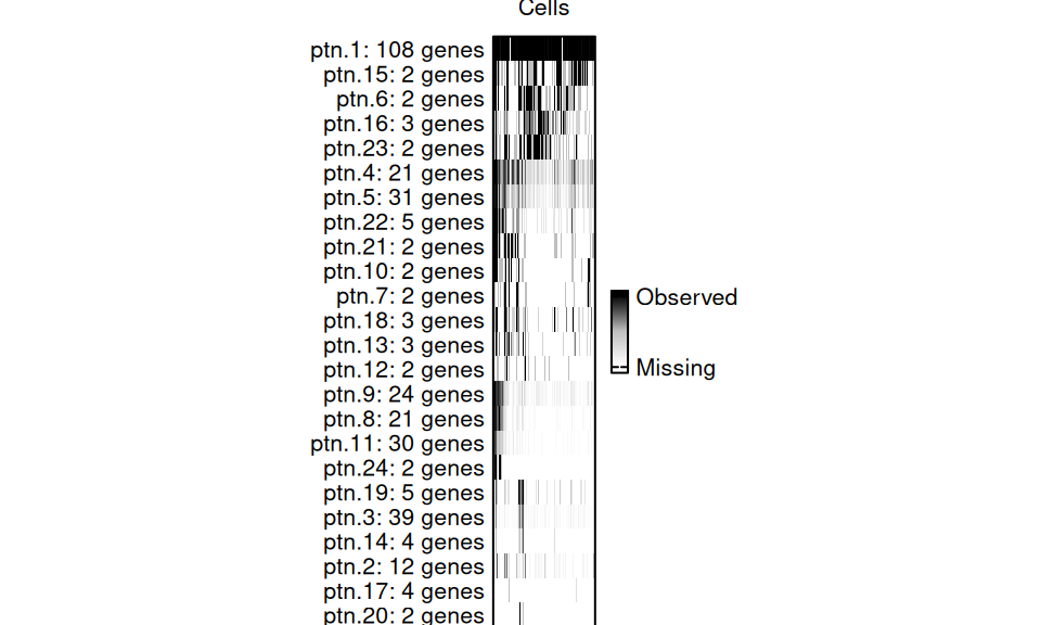
CGP Plot
For this dataset, we identified 24 sets of genes. Each slice of the bar represents a cell, and it is colored based on what percentage of genes from that pattern are expressed in each cell.
To get a data.frame of the genes within each pattern, use:
gcp <- get_pattern_genes(oar_obj)It is also possible to retrieve patterns when
oar_by_factor() is applied. Please see the documentation
for get_pattern_genes() for more details. Currently, the
oar_gcp_plot() is not supported when
oar_by_factor() is executed.
Score projection with Seurat FeaturePlot
As the scores, p values and sparsity have been added as columns to
the meta.data of the Seurat object, you can use all the
native functions from that package to visualize your results.
Seurat::FeaturePlot() in particular, is a good starting
point to get an overview of how the score is distributed among cells and
clusters.
library(Seurat)
#> Loading required package: SeuratObject
#> Loading required package: sp
#> 'SeuratObject' was built under R 4.5.0 but the current version is
#> 4.5.3; it is recomended that you reinstall 'SeuratObject' as the ABI
#> for R may have changed
#>
#> Attaching package: 'SeuratObject'
#> The following objects are masked from 'package:base':
#>
#>     intersect, t
p4 <- FeaturePlot(
  oar_obj, features = "OARscore", order = T, pt.size = 0.5,
  min.cutoff = "q40", max.cutoff = "q90")
p4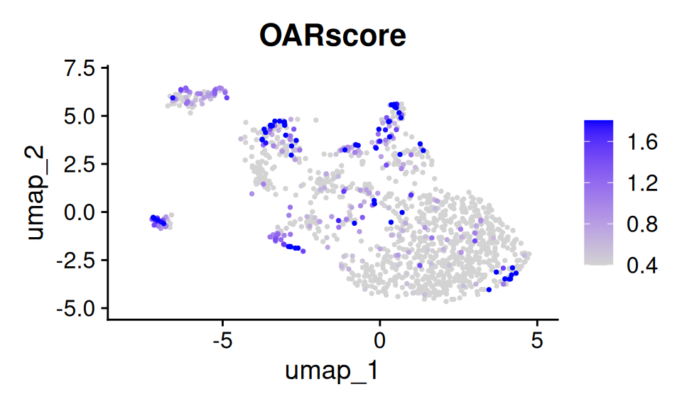
Feature plot of results
Starting from a Gene Expression Matrix
The steps to analyse a gene count matrix, with cells as columns and genes as rows, are very similar to what we saw above.
data <- readRDS(file = "pdcs_matrix.rds")Analysis
Once you have data loaded, you can run the oar function. In addition
to the input data we must specify that we are not starting with a Seurat
object by setting seurat_v5 to FALSE.
oar_data<- oar(data, seurat_v5 = FALSE,
               cores = 1)
#> Warning in oar(data, seurat_v5 = FALSE, cores = 1): Running process in fewer than 2 cores will considerably slow down progress
#> [1] "Extracting data..."
#> [1] "Analysis started on:"
#> [1] "2026-03-26 16:30:33 UTC"
#> [1] "Identifying gene co-expression patterns..."
#> [1] "Calculating Hamming distances between gene vectors using specified cores."
...
oar_data
#>           OARscore    KW.pvalue KW.BH.pvalue sparsity
#> 1     0.4991194964 1.310249e-74 1.672114e-74 79.46352
#> 2    -0.5335102274 9.891672e-83 3.595131e-82 87.92927
#> 3    -1.0294046721 7.161214e-87 7.474225e-86 85.27251
#> 4    -1.3317223078 2.258655e-89 4.253800e-88 78.79720
...
This results in a table with the following columns:
-
OARscoreis a metric of transcriptional shifts in the data, with a higher OAR score highlighting cells with gene expression patterns dissimilar from all others tested. -
KW.pvalueis the p-value generated by Kruskal-Wallis test. -
KW.BH.pvalueis the Benjamini-Hochberg corrected p-value. -
sparsityis the percent of genes in each cell with a count of 0.
Visualize Results
We can visualize these OAR scores with a scatter plot against sparsity.
p5 <- scatter_score(oar_data, seurat_v5 = F)
p5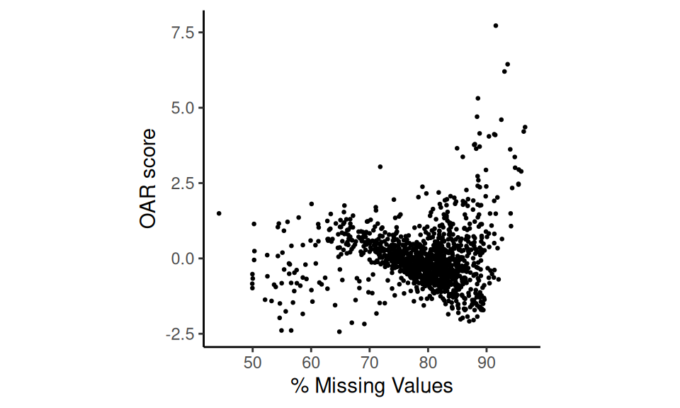
Scatter plot of results